Finding the Sides of Things

What makes a face a face — and why millimetres and degrees must never share a ruler

Carlos Valero Valdés

Look at a staircase and you have no trouble saying it has ten sides. Ask a computer, and the question turns out to have two halves that pull in different directions. A side is a patch where the surface points the same way — that is a statement about direction. But two treads point the same way and are still two sides — that is a statement about position. Getting both at once means clustering in two spaces simultaneously, and the moment you try, you hit a small scandal: a distance in millimetres and a distance in degrees cannot be added. The fix is a product kernel with one bandwidth per factor, and it is worth seeing what happens to people who skip it.

1. What is a side?

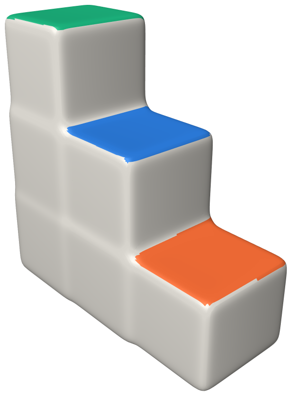
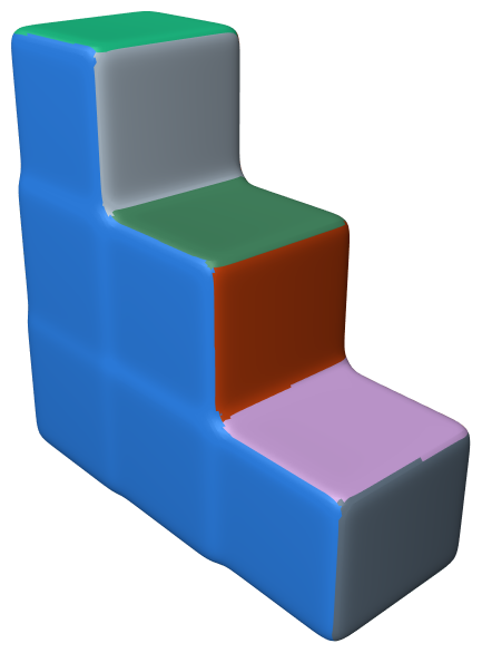
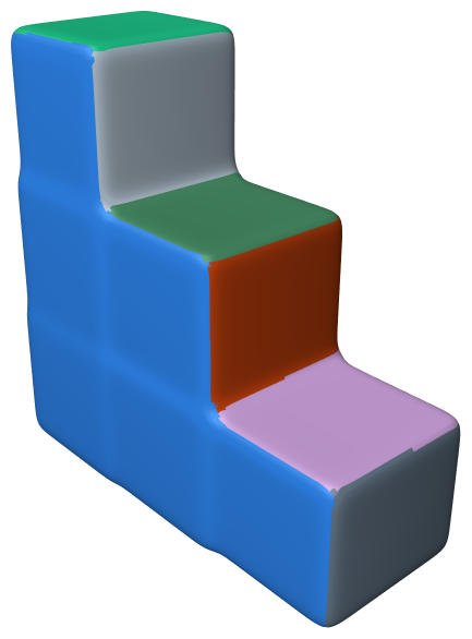
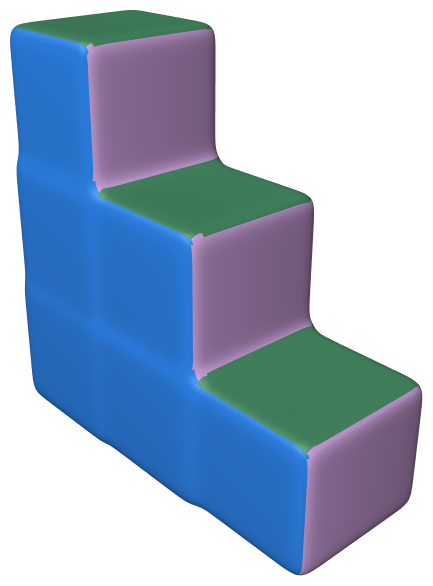
Here is a staircase. Not a real one — a solid with three steps, its edges slightly rounded the way a moulded or machined part’s edges always are.

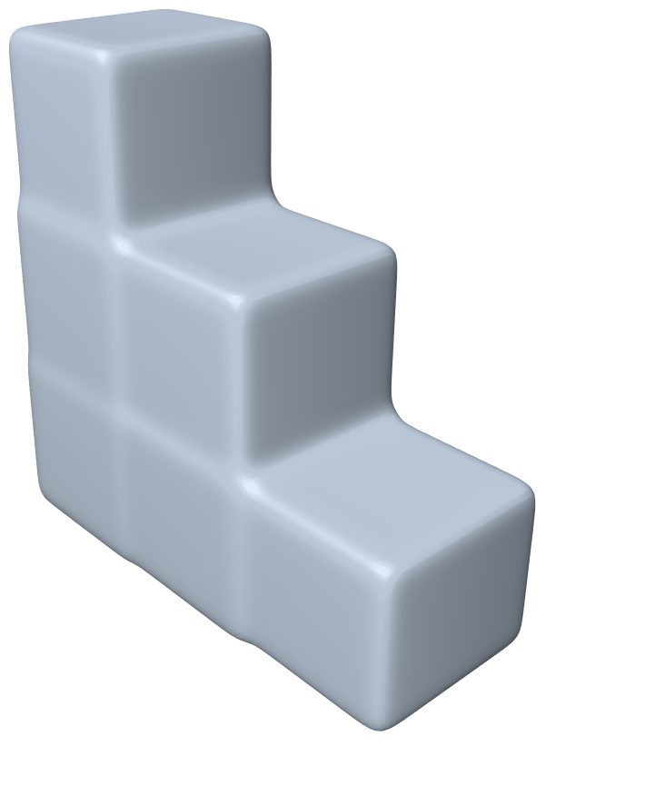
A three-step staircase solid with slightly rounded edges — Figure 1. Three treads, three risers, a tall face on each side, a back and a bottom: ten sides, and you counted them without being told how. The question is what rule you used.

Whatever the rule is, it is not about position alone — a side spans a wide stretch of space, and two adjacent sides meet along an edge where their points are as close together as points can get. And it is not about colour, or curvature, or connectivity. The thing that is constant across a side and changes as you step off it is the direction the surface faces.

2. The Gauss map

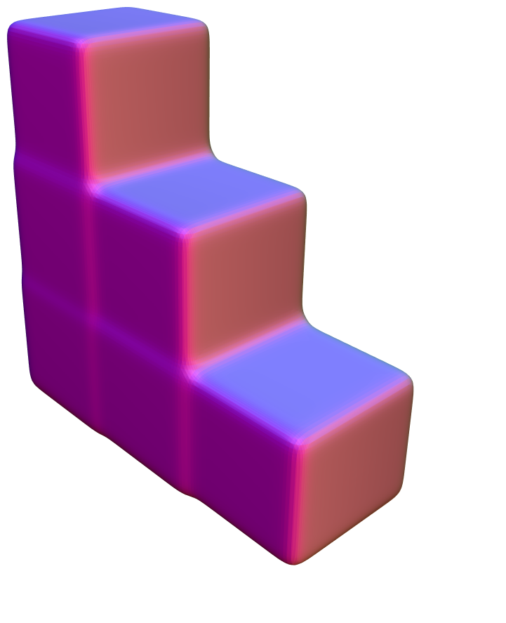
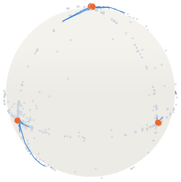
Give every little patch of the surface its outward normal — the unit arrow pointing straight away from it — and you have a map from the object to the unit sphere. It is called the Gauss map, and it is the natural home of the question.

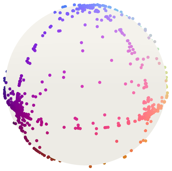
Under it, a flat face collapses to a single point: every patch of the top tread has exactly the same normal, so the whole tread lands on the north pole of the sphere and stays there. A rounded edge, by contrast, smears out into an arc, because its normal swings through a quarter turn as you cross it. So on the sphere, flat faces are spikes and roundings are smears — and finding the sides starts to look like finding the spikes.

The staircase with each face coloured by the direction of its normal — Figure 2. Left, every facet painted by its normal direction; right, those normals as points on the unit sphere, sampled in proportion to area. Six dense knots — the six directions the staircase’s flats face — joined by thin arcs, which are the rounded edges in transit between them. The knots are what we want.

The normals of the staircase plotted as points on a sphere, forming six tight clusters joined by faint arcs — Figure 2. Left, every facet painted by its normal direction; right, those normals as points on the unit sphere, sampled in proportion to area. Six dense knots — the six directions the staircase’s flats face — joined by thin arcs, which are the rounded edges in transit between them. The knots are what we want.

3. Six knots, ten sides

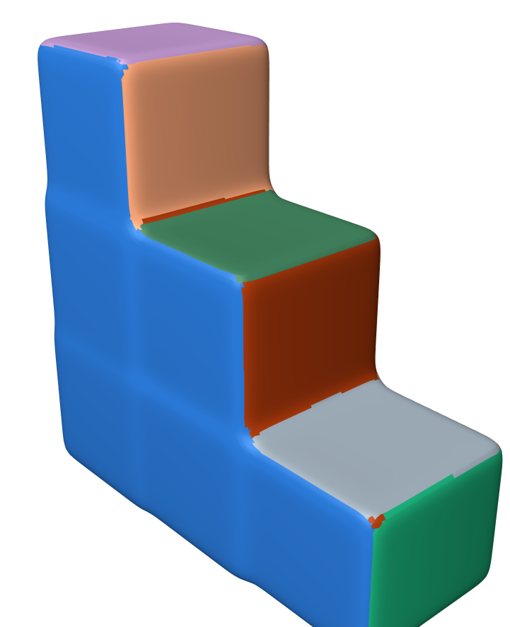
Cluster those normals and you will find six groups, because the staircase’s flats face in only six directions. But the staircase has ten sides. The three treads all face straight up; on the sphere they land on the same spot and are, as far as the Gauss map is concerned, one thing.

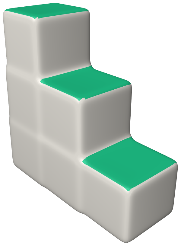
All three treads painted the same colour by normal-only clustering — Figure 3. The three treads, highlighted. Clustering on the sphere alone (left) finds six sides and paints all three treads with one colour: they really are indistinguishable by direction. Adding position (right) gives them three. The rest of the object is greyed out so the treads are easy to follow.

The three treads painted three different colours by joint clustering — Figure 3. The three treads, highlighted. Clustering on the sphere alone (left) finds six sides and paints all three treads with one colour: they really are indistinguishable by direction. Adding position (right) gives them three. The rest of the object is greyed out so the treads are easy to follow.

The obvious repair is to use position as well — but position alone is no better. Two facets straddling the nose of a step are millimetres apart and belong to different sides; two facets at opposite ends of one tread are far apart and belong to the same one. Neither coordinate works by itself. A side is a cluster in both at once: a patch whose facets agree about direction and sit near one another.

4. Two spaces, two rulers

So we cluster in the joint space of surface elements: each facet contributes a pair \((p, n)\) — a point in \(\RR^3\) and a point on \(S^2\). To cluster anything, we need to say how much weight a data point at \((p_i, n_i)\) carries as seen from \((p, n)\). Write it as a product:

\[ K\bigl((p, n), (p_i, n_i)\bigr) \;=\; \underbrace{\exp\!\left(-\frac{\lVert p - p_i \rVert^{2}}{2 h_p^{2}}\right)}_{\text{a length}} \;\cdot\; \underbrace{\exp\!\left(-\frac{\theta(n, n_i)^{2}}{2 h_n^{2}}\right)}_{\text{an angle}} , \]

where \(\theta(n, n_i)\) is the angle between the two normals. The two factors never mix. \(h_p\) is a distance, measured in whatever units the model is in; \(h_n\) is an angle, measured in degrees. Each says something you can state out loud:

\(h_n\) says how flat is flat — how far two normals may differ before the patches count as facing different ways.
\(h_p\) says how far is far — how much space may separate two patches that agree about direction before they count as different sides.

That the kernel factorises is not a convenience. It is the only honest thing to do, because there is no exchange rate between millimetres and degrees. We will come back to what happens to people who invent one.

5. Walking uphill

With a kernel in hand, mean shift is almost embarrassingly simple. Think of the kernel as smearing each data point into a small mound; the mounds pile up into a landscape, and the peaks of that landscape are the clusters. To find which peak you are under, you climb: replace your current position by the kernel-weighted average of the data around you, and repeat. You drift uphill and stop at the top. Everything that stops at the same summit is one cluster.

In the joint space each step does two averages. The position part is an ordinary weighted mean of points in space. The direction part cannot be — the average of two unit arrows is not a unit arrow, and the average of three arrows pointing at three corners of the sphere is a stubby thing pointing nowhere in particular. What you want is the mean direction: add the arrows as vectors and then renormalise to unit length.

Eighty paths on the sphere, each starting at a scattered normal and converging to one of six modes — Figure 4. Eighty seeds climbing, drawn on the sphere of directions — only the direction half of each path is shown. The pale dots are the data: the staircase’s normals. Each blue trail is one seed walking uphill; the clay dots are where they stop. Seeds that begin on the smeared arcs — the rounded edges — slide off them and fall into whichever flat face is nearer, which is exactly the behaviour you want from a roundover.

Run this from every facet, collect the summits, and the staircase comes apart into its sides — ten of them, one colour each.

The staircase segmented into ten sides, each in a distinct colour — Figure 5. Ten sides, found with \(h_n = 15°\) and \(h_p = 0.35\) in model units. Three treads, three risers, the long face down the near side, the tall back, the far end and the underside. The rounded edges have been absorbed into their neighbours rather than becoming sides of their own.

6. Turning the two knobs

Because the bandwidths mean separate things, they can be reasoned about separately — which is the practical payoff of keeping the kernel a product.

Open \(h_n\) and the method grows more tolerant about direction. Too tight and the rounded edges stop being transitional and start being sides of their own; too loose and faces that genuinely point different ways get swept together.

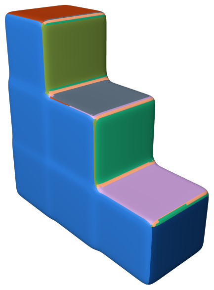
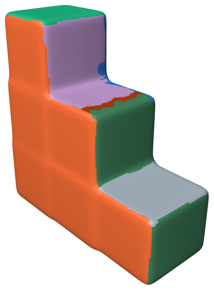
Segmentation at 5 degrees: thirteen sides — Figure 6. Sweeping the angular bandwidth with \(h_p\) held at 0.35. At 5° the roundovers survive as slivers of their own; at 15° they are absorbed and the count is right; at 45° the method has stopped caring which way things face and begins merging across corners.

Segmentation at 15 degrees: ten sides — Figure 6. Sweeping the angular bandwidth with \(h_p\) held at 0.35. At 5° the roundovers survive as slivers of their own; at 15° they are absorbed and the count is right; at 45° the method has stopped caring which way things face and begins merging across corners.

Open \(h_p\) and the method grows more tolerant about distance — and here the behaviour at the far end is worth dwelling on. Push \(h_p\) to infinity and the position factor becomes the constant 1: the kernel degenerates into pure direction clustering, and the answer collapses back to the six knots of the Gauss map. Section 3’s failure was never a different method. It was this one, with a knob turned all the way up.

Segmentation at position bandwidth 0.22: sixteen sides — Figure 7. Sweeping the position bandwidth with \(h_n\) held at 15°. Too small and single faces fracture into pieces; in the middle the answer is right; at the limit the position factor drops out and only the six directions remain.

Segmentation at position bandwidth 0.35: ten sides — Figure 7. Sweeping the position bandwidth with \(h_n\) held at 15°. Too small and single faces fracture into pieces; in the middle the answer is right; at the limit the position factor drops out and only the six directions remain.

7. The trap

Now the part that makes the product structure worth insisting on. It is tempting to flatten each facet into a single six-number vector, \((x, y, z, n_x, n_y, n_z)\), hand the pile to an off-the-shelf clustering routine, and give it one bandwidth. People do this. It appears to work.

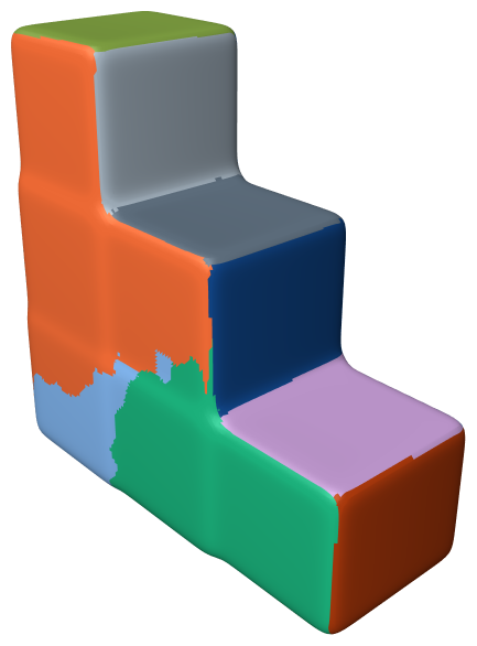
It appears to work because a single bandwidth silently declares an exchange rate: it says that one unit of distance is worth one unit of normal-vector difference. Normals are unit vectors, so their differences are always between 0 and 2, fixed once and for all. Distances are not — they are whatever your file says they are. Load the same part in millimetres instead of centimetres and every position coordinate grows by ten while every normal coordinate stays put. The exchange rate has moved by a factor of ten, and nobody has said anything.

Single-bandwidth clustering at one scale: ten clusters — Figure 8. One bandwidth on the six-vector, applied to the same staircase in two sets of units. On the left it happens to give the right answer. On the right, with nothing changed but the number printed on the ruler, it shatters into 127 fragments. The product kernel run on the same two models returns identical labels, facet for facet, because scaling the model and scaling \(h_p\) with it leaves the position factor untouched and never touches the angular one at all.

Single-bandwidth clustering at four times the scale: 127 clusters, a confetti of fragments — Figure 8. One bandwidth on the six-vector, applied to the same staircase in two sets of units. On the left it happens to give the right answer. On the right, with nothing changed but the number printed on the ruler, it shatters into 127 fragments. The product kernel run on the same two models returns identical labels, facet for facet, because scaling the model and scaling \(h_p\) with it leaves the position factor untouched and never touches the angular one at all.

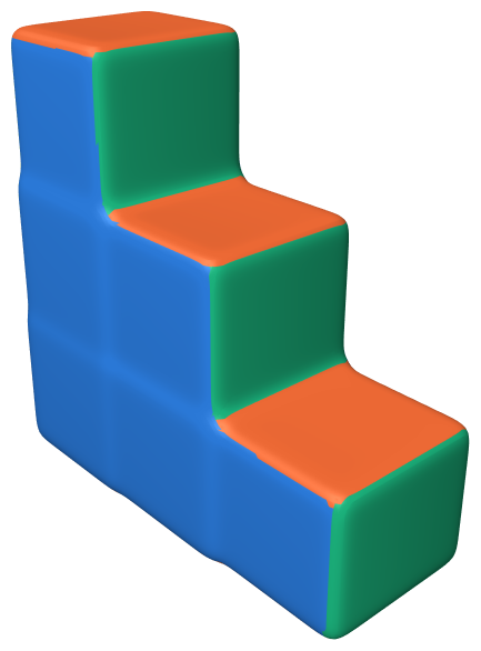
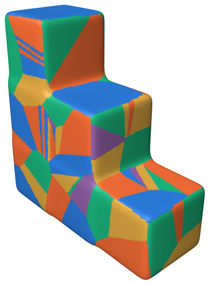
The left-hand picture is the dangerous one. A method that is wrong everywhere gets fixed. A method that is meaningless but right on your test file gets shipped.

8. Where it runs out

Honest accounting. The two bandwidths have to satisfy conflicting demands, and on some objects no value satisfies both. \(h_p\) must be large enough that one face is a single mound rather than a plateau with several bumps — which means comparable to the face’s own width. It must also be small enough to keep two faces that share a normal from merging — which means smaller than the gap between them. If a face is wider than its distance to the next face pointing the same way, there is no such \(h_p\).

The bracket from the previous article is exactly that case. Its base plate is 1.9 units across, and the arm directly above it is 1.38 units away — the face is wider than the gap.

The bracket with a small position bandwidth: the two tops are separate colours but the base top is split in two — Figure 9. The same two upward-facing sides on the bracket, in clay and blue. At \(h_p = 0.35\) they are told apart, but the base plate’s top breaks into two pieces. At \(h_p = 0.7\) the base top is whole again — and has swallowed the arm top, so both are clay. There is no setting that does both, and the staircase works only because every one of its faces is small compared with the distance to the next face facing the same way.

The bracket with a larger position bandwidth: the base top is whole but has merged with the arm top — Figure 9. The same two upward-facing sides on the bracket, in clay and blue. At \(h_p = 0.35\) they are told apart, but the base plate’s top breaks into two pieces. At \(h_p = 0.7\) the base top is whole again — and has swallowed the arm top, so both are clay. There is no setting that does both, and the staircase works only because every one of its faces is small compared with the distance to the next face facing the same way.

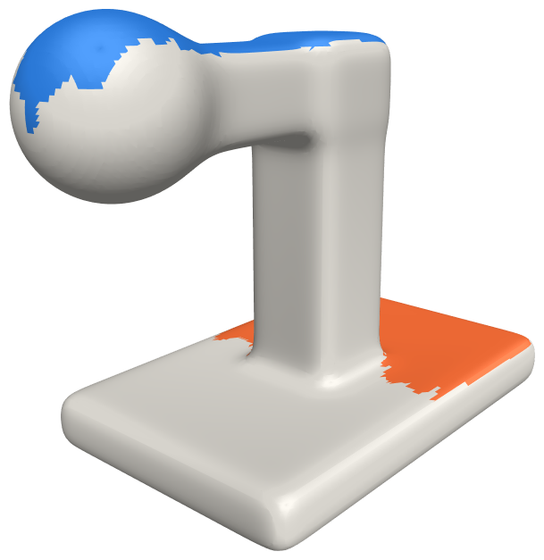
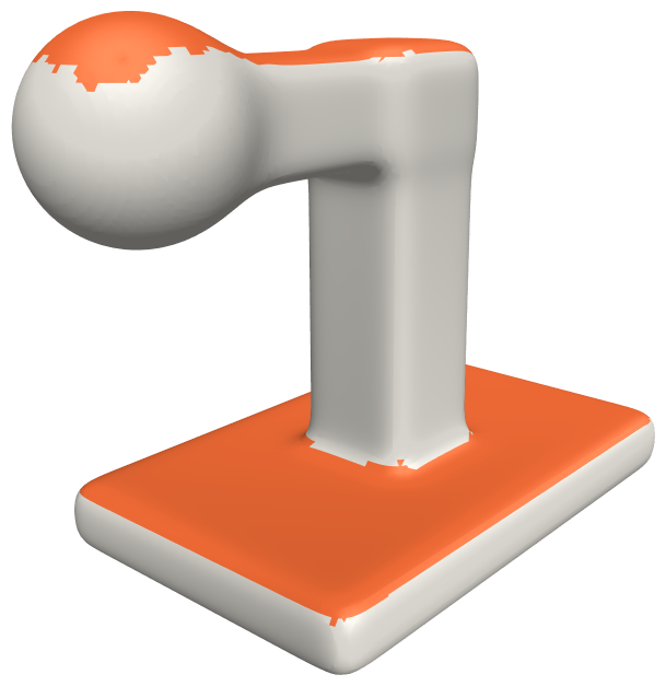
There is a second limit in the same family. Mean shift finds peaks, so it can only report a side that has a peak. A ring-shaped face — the top of a plate with a post through the middle — has a hole where its centre should be, and a hole is not a peak. The method reports such a face in pieces, and it is not being stupid: it is answering the question it was asked, which was about the modes of a density and not about connected components of a surface.

9. Try it

One step of the climb, in full. The weights are the product; the position update is an average; the direction update is an average followed by a renormalisation:

def step(p, n, P, N, w, h_p, h_n):
    """One mean-shift step from (p, n) through the data (P, N)."""
    k  = np.exp(-0.5 * ((P - p)**2).sum(1) / h_p**2)      # a length
    k *= np.exp(-0.5 * (np.arccos((N @ n).clip(-1, 1)) / h_n)**2)   # an angle
    k *= w                                                 # facet areas

    p_new = (k[:, None] * P).sum(0) / k.sum()              # mean point
    v     = (k[:, None] * N).sum(0)                        # mean direction,
    return p_new, v / np.linalg.norm(v)                    #   back on S^2

The two bandwidths appear on two separate lines and are never compared with one another. The accompanying tests check that this is not merely tidy: that the kernel factorises exactly, that renormalising really does minimise what it is supposed to, that an exact cube yields exactly six sides with exactly axis-aligned normals and exactly equal areas, that the staircase yields ten with its treads apart, that normals alone yield six with its treads together, and that rescaling the model leaves every label untouched while the single-bandwidth version goes from eleven clusters to ninety-nine.

The moral is about units, and it outlives this problem. Whenever a method wants a distance and your data has parts measured in different things — metres and degrees, dollars and days, pixels and seconds — concatenating them into one vector does not combine them. It hides an arbitrary conversion factor inside a norm, where nobody will look for it. A product of kernels drags the factor into the open and makes you name it, once per space, in the units that space actually uses.