When Geometry Acts Like a Force

A molecule loose in a narrow channel is pushed by nothing at all — and still climbs hills

Carlos Valero Valdés

A protein threading a nuclear pore, an ion crossing a membrane channel, a bead in a microfluidic duct: something small, loose inside something narrow, shoved about at random and heading nowhere in particular. Usually all you want to know is how far along it has got, so you throw away two of the three coordinates — and the throwing away leaves a residue. In a channel that bulges and pinches, the wanderers pile up in the bulges and stay there, permanently, with no force anywhere in the picture. Written down, that residue is an ordinary potential landscape assembled out of nothing but the logarithm of the available room. This is the Fick–Jacobs equation. Here it is built up from pictures, and then pushed until it breaks.

1. A molecule in a pore

Start with the picture, not the equation. Something small is loose inside something narrow: a protein threading a nuclear pore; an ion crossing a channel in a cell membrane, perhaps a nanometre across; a dye molecule working its way through the pore network of a rock; a bead in a microfluidic channel ten micrometres wide.

None of these wanderers are being pumped. The molecule is jostled by the solvent around it, millions of times a second, from every direction at once. It has no heading and no memory: over a short interval it is as likely to step one way as the other. That is Brownian motion, and on its own it is well understood.

What makes the problem interesting is that the container is not a straight pipe. Real channels bulge and pinch. And the shape of the container turns out to change the answer in a way that has nothing to do with forces.

2. One number instead of three

To describe the molecule exactly you would track a probability cloud \(P(x, y, z, t)\) filling a complicated three-dimensional region, with the condition that nothing leaks through the walls. That is a hard problem, and usually far more than you wanted — because in practice you rarely care about the molecule’s height, or its distance from the wall. You care how far along it has got. How long until it reaches the other side? Where is it likely to be after a millisecond? Those are questions about one coordinate: the position \(x\) along the channel’s axis.

So the natural move is to squash the cloud onto the axis. At each station \(x\), add up all the probability sitting in that cross-section:

\[ p(x, t) \;=\; \int_{\Omega(x)} P(x, y, z, t)\,\mathrm{d}y\,\mathrm{d}z . \]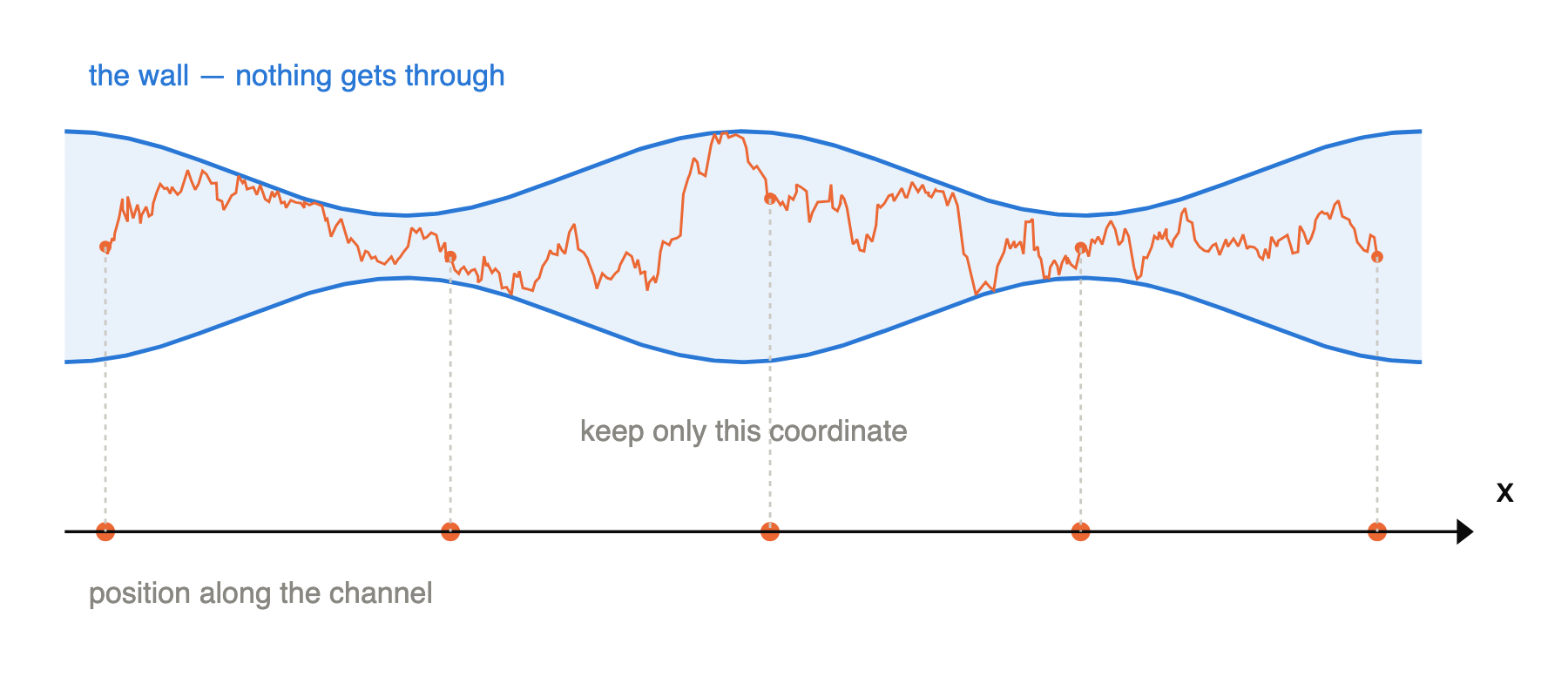

A wandering path inside a bulging channel, with five of its positions dropped onto an axis below — Figure 1. The molecule wanders in three dimensions; only its progress along the axis is recorded. Everything the walls do to it has to survive this flattening, which is the whole difficulty.

The question is what equation \(p(x, t)\) obeys. That equation is the Fick–Jacobs equation, and the surprise is that it is not the obvious one.

3. Why plain diffusion is the wrong answer

The obvious guess is that squashing a diffusion problem gives back a diffusion problem:

\[ \frac{\partial p}{\partial t} \;=\; D\,\frac{\partial^{2} p}{\partial x^{2}} , \]

which is right for a pipe of constant width and wrong for everything else. The way it fails is the key to all that follows.

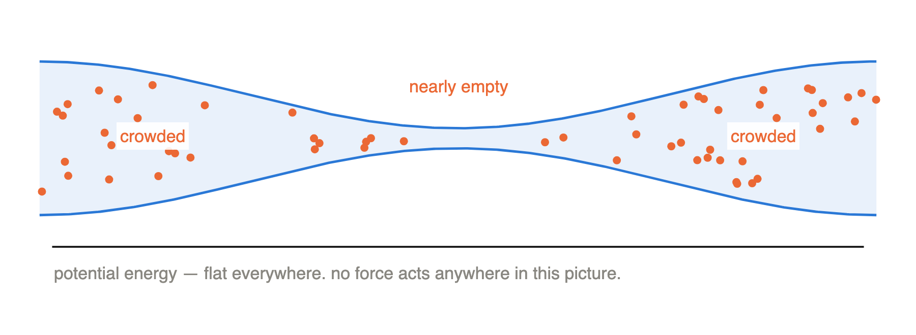
Release a great many molecules into a bulging channel and wait until nothing changes any more. In a straight pipe they end up spread perfectly evenly, which is what plain diffusion predicts. In a bulging pipe they do not. They pile up in the wide parts and thin out in the narrow ones — permanently, as the settled state, not as a passing phase.

Nothing is pulling them into the bulges. There is no field, no charge, no attraction to the walls. There is simply more room there, and a wanderer with no preferences spends its time in proportion to the room available.

Particles gathered in the two wide ends of a channel and nearly absent from its neck — Figure 2. Every position here has identical energy, so no force exists anywhere in the picture. The particles still gather in the chambers, purely because there are more places to be. This is the entire effect that plain diffusion along a line cannot represent.

That is a claim about what happens, so here it is happening. Six hundred walkers take genuinely random steps inside a corrugated channel — no forces, no bias, nothing but a wall that reflects them. The bars underneath count how much time they spend at each position.

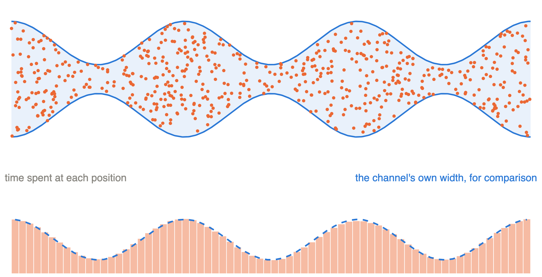
Simulated walkers in a corrugated channel, with a histogram of time spent that follows the channel's width — Figure 3. Six hundred reflecting walkers, and the time they spend at each station. The dashed curve is not fitted to the bars: it is the channel’s own half-width, drawn on the same axes. Occupancy settles proportional to the width — in three dimensions, proportional to the cross-sectional area. Nothing in the simulation knows anything about the channel except that it bounces.

One detail of that simulation is worth flagging now, because the whole article turns on it. A walker that steps through the wall is mirrored back in, and the mirror is the wall’s tangent plane. Wherever the channel is widening or narrowing, that plane is tilted with respect to the axis, so a bounce moves the walker along the channel as well as across it. Reflect only the crosswise coordinate — the tempting shortcut — and the axial motion never feels the channel at all: the walkers stay spread perfectly evenly no matter what shape you put them in, and the figure above comes out flat. The tilt of the wall is not a detail. It is the mechanism.

4. Room becomes a force

Write \(A(x)\) for the cross-sectional area at station \(x\). What the simulation shows is that, once everything has settled, \(p(x) \propto A(x)\): occupancy simply follows available room.

Now compare that with how a particle settles in a landscape of real forces. There, statistical mechanics gives the Boltzmann distribution — the chance of being somewhere falls off exponentially with the energy there, \(p \propto e^{-F/k_{B}T}\). Set the two side by side, solve for \(F\), and something worth pausing over drops out:

\[ F(x) \;=\; -\,k_{B}T \ln A(x) . \]

The particle behaves exactly as if it were moving through a potential landscape, and that landscape is nothing but the logarithm of the room available at each station. A pinch becomes a hill. A bulge becomes a valley. The molecule is pushed by nothing at all and still climbs and descends.

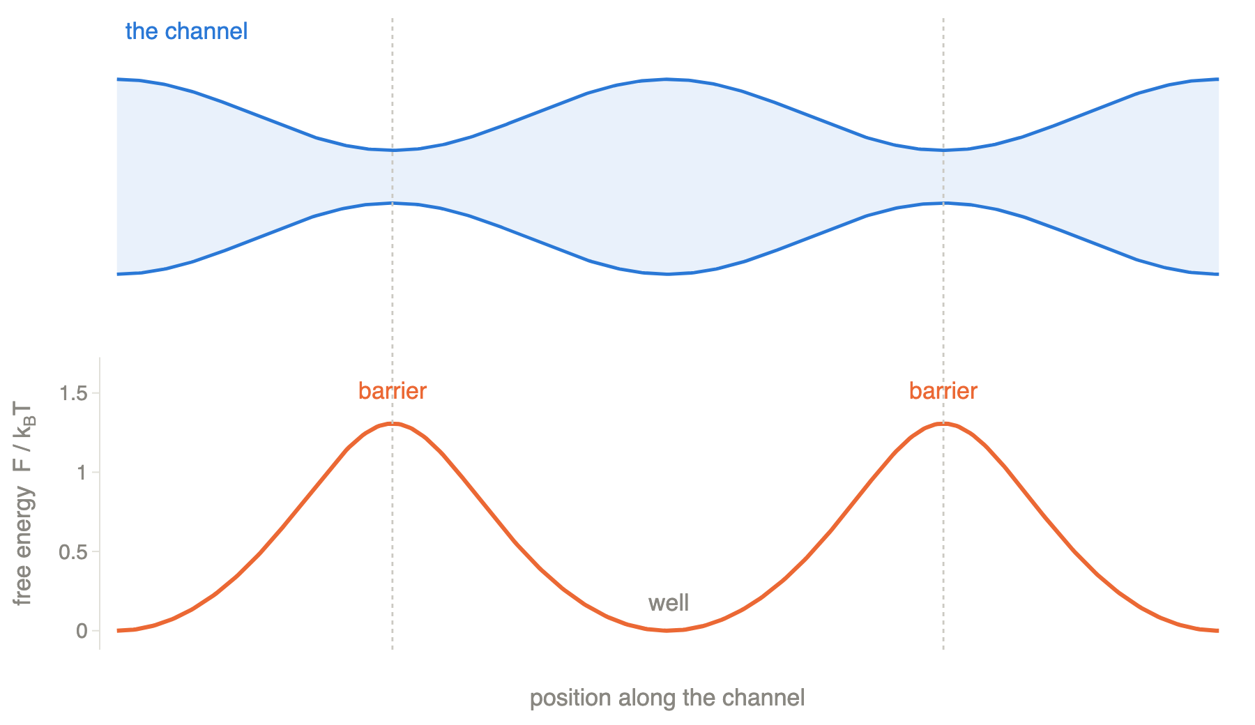
A corrugated channel above, and below it the free energy minus log of its width, with barriers at the pinches — Figure 4. Geometry, drawn as a landscape. The dotted guides mark the pinches; each one sits under a hill in the free energy. The two are the same picture — the lower curve is the logarithm of the upper one, turned upside down.

This is called an entropic barrier, and the name is precise: the obstacle is made of missing options rather than of energy. Squeezing through a neck costs the molecule not effort but opportunity. There are very few ways to be inside a neck and overwhelmingly many ways to be inside a chamber, and a wanderer that has no preferences is therefore rarely in the neck — which, seen from the axis, is indistinguishable from being pushed out of it.

5. The equation, read slowly

Here it is. It looks more elaborate than plain diffusion, but every piece is doing an identifiable job.

\[ \frac{\partial p}{\partial t} \;=\; \frac{\partial}{\partial x} \left[\, D(x)\,A(x)\,\frac{\partial}{\partial x}\!\left(\frac{p}{A(x)}\right)\right] \]

\(p/A\) is the concentration, and it is the crux. \(p\) counts particles in a slice; dividing by the area converts it to particles per unit volume. A fat slice can hold a great many particles at low concentration. Diffusion responds to concentration, not to headcount, so this ratio — not \(p\) itself — is what must be differentiated.
\(\partial(p/A)/\partial x\) is the driving gradient: Fick’s law, correctly applied. Flow runs from higher concentration to lower. If the concentration is uniform this is zero and nothing moves, however lumpy \(p\) itself may be.
\(A(x)\) is the size of the opening. It converts a flux per unit area into the total flow crossing that station: a wide cross-section passes more at the same gradient.
The outer \(\partial/\partial x\) is bookkeeping. Whatever flows in and does not flow out has to accumulate. It is conservation of particles, nothing more.

There is an equivalent way to write it that makes the landscape explicit. Using \(F = -k_{B}T \ln A\), the same equation becomes an ordinary drift-and-diffusion equation in that entropic landscape:

\[ \frac{\partial p}{\partial t} \;=\; \frac{\partial}{\partial x} \left[\, D\left(\frac{\partial p}{\partial x} + \frac{p}{k_{B}T}\,\frac{\partial F}{\partial x}\right)\right] . \]

Two faces of one equation. The first says concentration drives flow through an opening of varying size; the second says the particle diffuses while sliding down an entropic hill. Expand the derivatives and they are the same expression, term for term.

6. The subtlety hiding in D

So far \(D\) has been carried along without comment. It is where the remaining difficulty lives, and where most of the research on this equation has gone.

Getting from three dimensions to one required an assumption that was never stated out loud: that at every instant the particle is spread evenly across the cross-section. Only then can a slice be described by its total \(p\) alone. That is never exactly true. Spreading across a channel takes time — roughly \(R^{2}/D_{0}\) for a channel of half-width \(R\) — and if the wall slopes, then advancing along the axis means the particle must also travel sideways to stay spread across the widening section. It is always slightly behind.

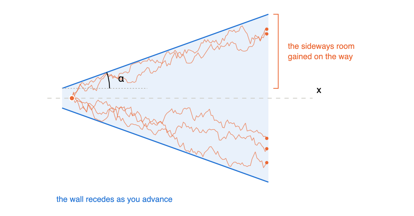
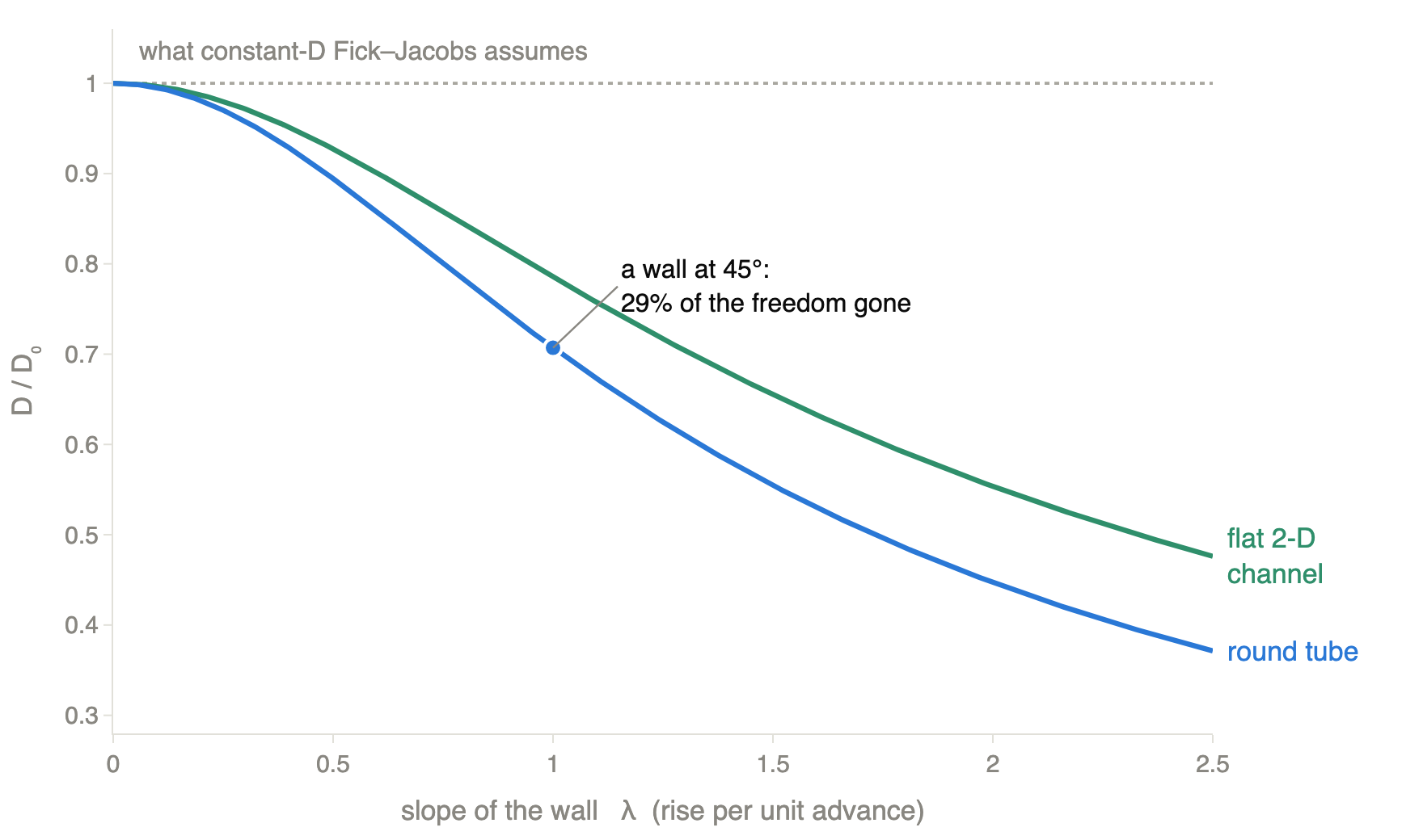
Five random paths spreading outwards as they advance along a widening cone, with the wall's angle marked — Figure 5. Keeping up costs something. Five walkers released together at the narrow end; to stay spread across the section they must travel the bracketed distance sideways as well as the whole length forward. Sideways spreading is not instantaneous, so the projected motion along the axis is slower than free diffusion would be.

The repair is to let the coefficient depend on position: \(D\) becomes \(D(x)\), smaller than the free value \(D_{0}\) wherever the wall is steep. Two closed forms cover most of what is used in practice. For a round tube of radius \(R(x)\), Reguera and Rubí give

\[ D(x) \;=\; D_{0}\left(1 + R'(x)^{2}\right)^{-1/2} , \]

which for a straight cone is exactly \(D_{0}\cos\alpha\), since \(\tan\alpha = R'\). For a flat two-dimensional channel of half-width \(w(x)\), the Kalinay–Percus resummation of the systematic expansion gives

\[ D(x) \;=\; D_{0}\,\frac{\arctan w'(x)}{w'(x)} . \]

Both equal \(D_{0}\) for a wall parallel to the axis and fall away as the wall steepens, but they fall at different rates — \(1 - \tfrac{1}{2}\lambda^{2}\) against \(1 - \tfrac{1}{3}\lambda^{2}\) for small slope \(\lambda\). The difference is dimensionality: a particle in a round tube has more sideways room to cover than one in a flat slit.

Two curves of D over D-zero falling with wall slope, against the flat line constant-D assumes — Figure 6. What the slope costs. Both coefficients are exactly \(D_{0}\) for a wall parallel to the axis and decline from there. At a slope of 1 — a wall at 45° — a round tube has already lost 29% of its free diffusivity. The dotted line is what constant-\(D\) Fick–Jacobs assumes throughout.

7. When to believe it

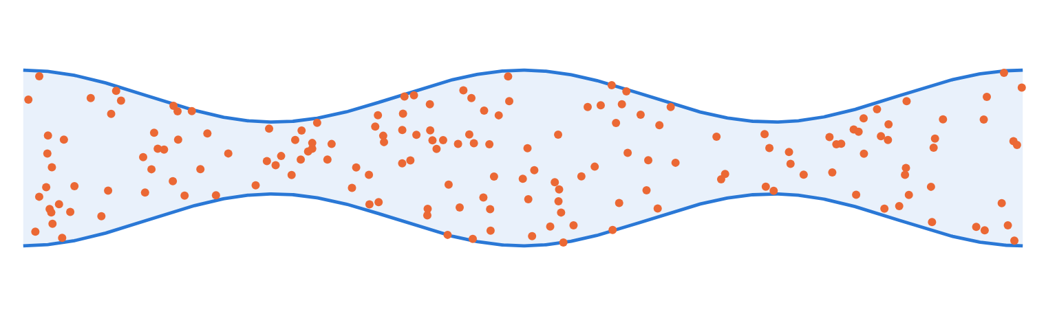
The equation is an approximation with a clearly marked domain, and it is worth knowing which side of the line a given channel falls on. It works well when the channel is narrow compared with the distance over which it changes shape — when the wall slope is small, say \(|R'| \lesssim 1\). Then sideways spreading really is fast compared with axial progress, which is the assumption the whole derivation rests on. Gently corrugated pores, tapered micro-channels and slowly flaring nozzles are all comfortably inside.

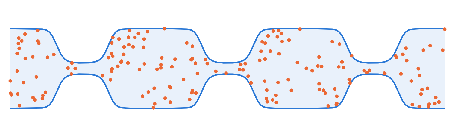
It struggles when the channel has abrupt steps or sharp corners, where the wall slope is effectively infinite and no expansion in it converges. Or when the geometry is a chain of large chambers joined by very short narrow necks — there the physics is better described as hopping between chambers at some rate than as diffusion along a coordinate. Or when the cross-section is so wide that a particle genuinely fails to explore it before moving on.

A gently corrugated channel with walkers spread in proportion to its width — Figure 7. Two channels, the same walkers. On the left the wall never exceeds 18°, and a coordinate along the axis is a fair description of where the particle is. On the right the necks are short and the walls nearly vertical: a particle in a chamber stays there for a long time and then makes a dash, which is a different kind of process wearing the same clothes.

Wide chambers joined by short narrow necks, with walkers almost absent from the necks — Figure 7. Two channels, the same walkers. On the left the wall never exceeds 18°, and a coordinate along the axis is a fair description of where the particle is. On the right the necks are short and the walls nearly vertical: a particle in a chamber stays there for a long time and then makes a dash, which is a different kind of process wearing the same clothes.

8. What area cannot see

Notice what both coefficients in Section 6 have in common: each depends only on how the cross-sectional area varies along the channel. Neither knows what shape the cross-section is. That turns out to be an incomplete accounting, and the cleanest way to show it is to build a channel where area has nothing at all to report.

Take a perfectly straight axis and a cross-section of constant area — an ellipse, say — and let that ellipse slowly rotate as you advance, like a twisted ribbon. The area never changes, so \(R' = 0\) everywhere and both formulas return the free value \(D_{0}\), with no penalty at all.

A tube with a straight axis whose elliptical cross-section rotates as it advances — Figure 8. Straight axis, constant area, turning section: two full turns over the length shown, with the section itself drawn at five stations. Every area-based effective coefficient reports that nothing whatever is happening here.

But the wall is not parallel to the axis. A particle out near the tip of the long axis finds that the tip swings away as it advances, so it must shuffle sideways to keep up — and by Section 6’s own argument, that must slow it down. Which is it: the formulas, or the argument?

This one can be settled. Walk twenty thousand particles through such a tube, with nothing acting on them but a reflecting wall, and measure how fast the cloud spreads along the axis. The section used below is an ellipse two units across and seven-tenths of a unit deep, and the twist rate says how many radians it turns through per unit of length travelled.

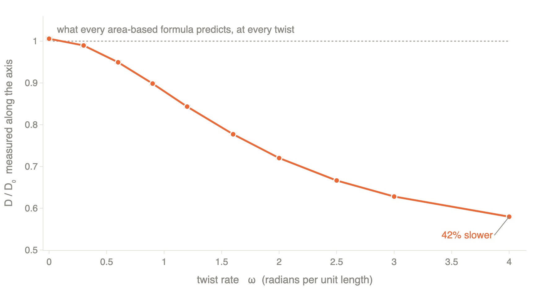
Measured axial diffusivity falling from 1 to 0.58 as the twist rate increases, against a flat prediction of 1 — Figure 9. Measured axial diffusivity against twist rate. At zero twist the tube is an ordinary elliptical cylinder and the measurement returns \(D_{0}\), as it must — that is the control. Turn the section once every five lengths and 16% of the diffusivity is gone; once every 1.6 lengths, about one channel width, and 42% is gone. The dotted line is what every area-based formula predicts at every twist rate on the plot. Error bars are smaller than the dots.

So the formulas are not merely imprecise here; they are blind. The same is true of a channel whose section keeps its area but changes shape as it advances, and of one that merely drifts off to one side while staying exactly the same size throughout. In each case the area-based coefficients predict that nothing happens, and something does. Recovering that missing suppression — the part of the geometry that area alone cannot see — is an active line of work, and it is why the coefficient wants to be written in terms of the channel’s geometry rather than its cross-sectional bookkeeping.

9. Try it

Every simulation in this article is the same four lines. A channel is anything that can say where its wall is: a function \(g\) that is negative inside, zero on the wall and positive outside, together with its gradient. A walker takes a free Brownian step; if it has left, it is mirrored back in.

def bounce(channel, q):
    """Mirror a walker that stepped through the wall back inside."""
    n = channel.grad(q)                      # points across the wall
    wall = q - (channel.g(q) / dot(n, n))[:, None] * n
    n = channel.grad(wall)                   # the normal where it left
    over = dot(q - wall, n) / dot(n, n)      # how far past it went
    return q - 2 * over[:, None] * n         # mirrored back inside

The normal \(n\) is the whole story. Whenever the wall is not parallel to the axis it has a component along the axis, and reflecting through it costs the walker axial progress. Delete that component — reflect only the crosswise coordinates, which is what it feels natural to do — and you have built a world in which the shape of a channel does not matter at all: walkers spread evenly through necks and chambers alike, and no amount of corrugation slows anything down. Every effect in this article lives in that one component.

The accompanying tests check what can be checked. That \(p \propto A\) makes the flux identically zero while an evenly spread \(p\) does not; that the two ways of writing the equation are the same expression to machine precision; that the round-tube coefficient is exactly \(D_{0}\cos\alpha\) for a cone and that the two small-slope expansions really are \(1-\lambda^{2}/2\) and \(1-\lambda^{2}/3\); that a reflecting walk settles into the channel’s own width to within 4%; that a turning circular section — a cylinder in disguise — gives back exactly \(D_{0}\), which is how you know the simulator has no axial bias of its own; and that a corrugated round tube lands within a few percent of what Fick–Jacobs predicts for it.

What stays with me is how much of this is bookkeeping about what you agreed to forget. The molecule never felt a force. It was only ever bouncing. The hill exists because we decided to write down one number instead of three, and the hill is exactly the price of that decision — payable in full, as long as the wall slopes gently and the section does not turn.